Monte Carlo Simulations in Finance

Introduction: Why Monte Carlo Methods Dominate Complex Valuation

In the realm of financial engineering, Monte Carlo (MC) simulations have emerged as the gold standard for pricing instruments where closed-form solutions fail. Unlike traditional models (Black-Scholes, binomial trees), MC methods excel at handling:

✔ Path-dependent payoffs (e.g., Asian options, barrier clauses)

✔ Multiple stochastic factors (equity prices, interest rates, weather variables)

✔ Early exercise features (convertible bonds, American options)

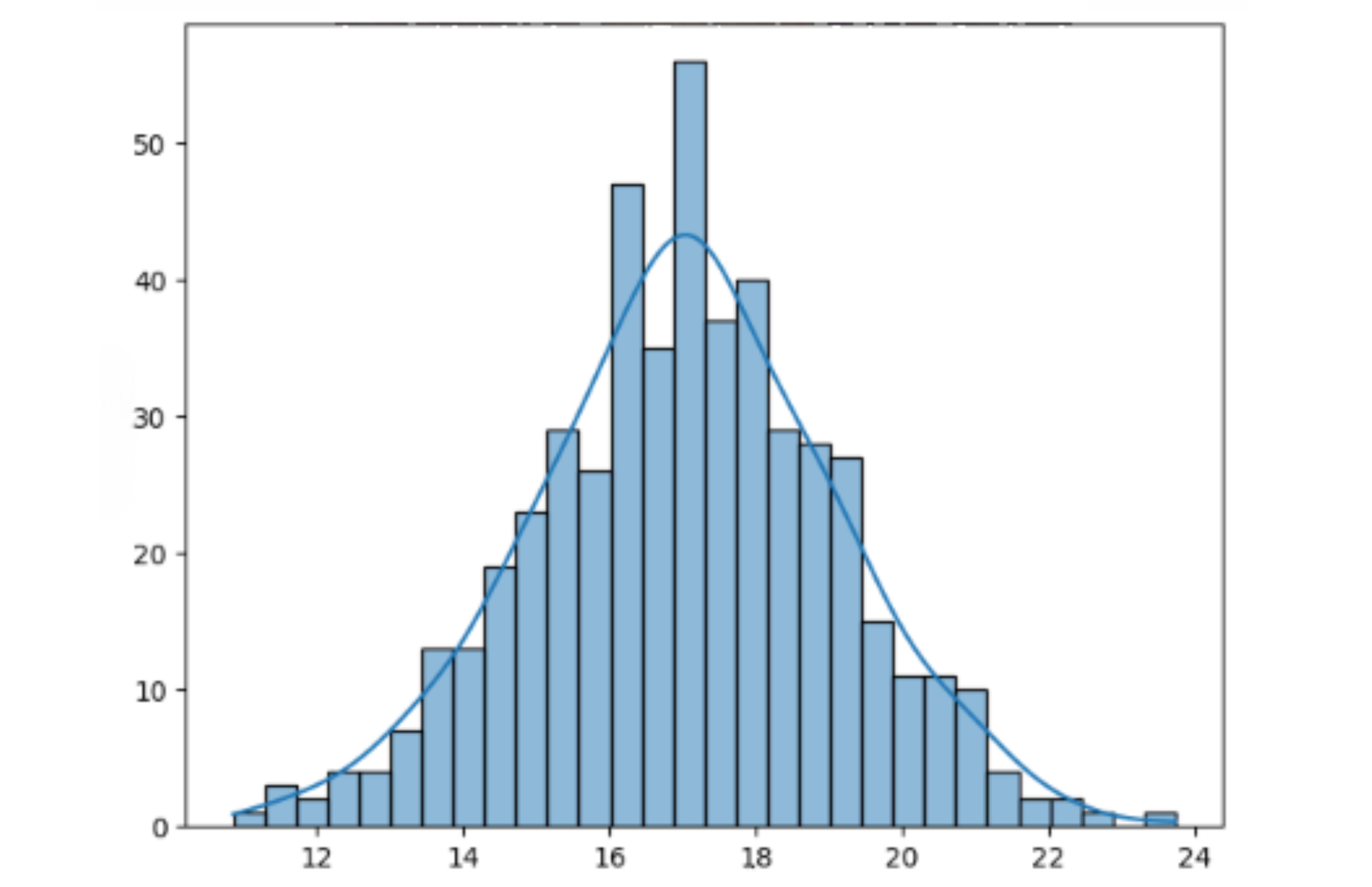
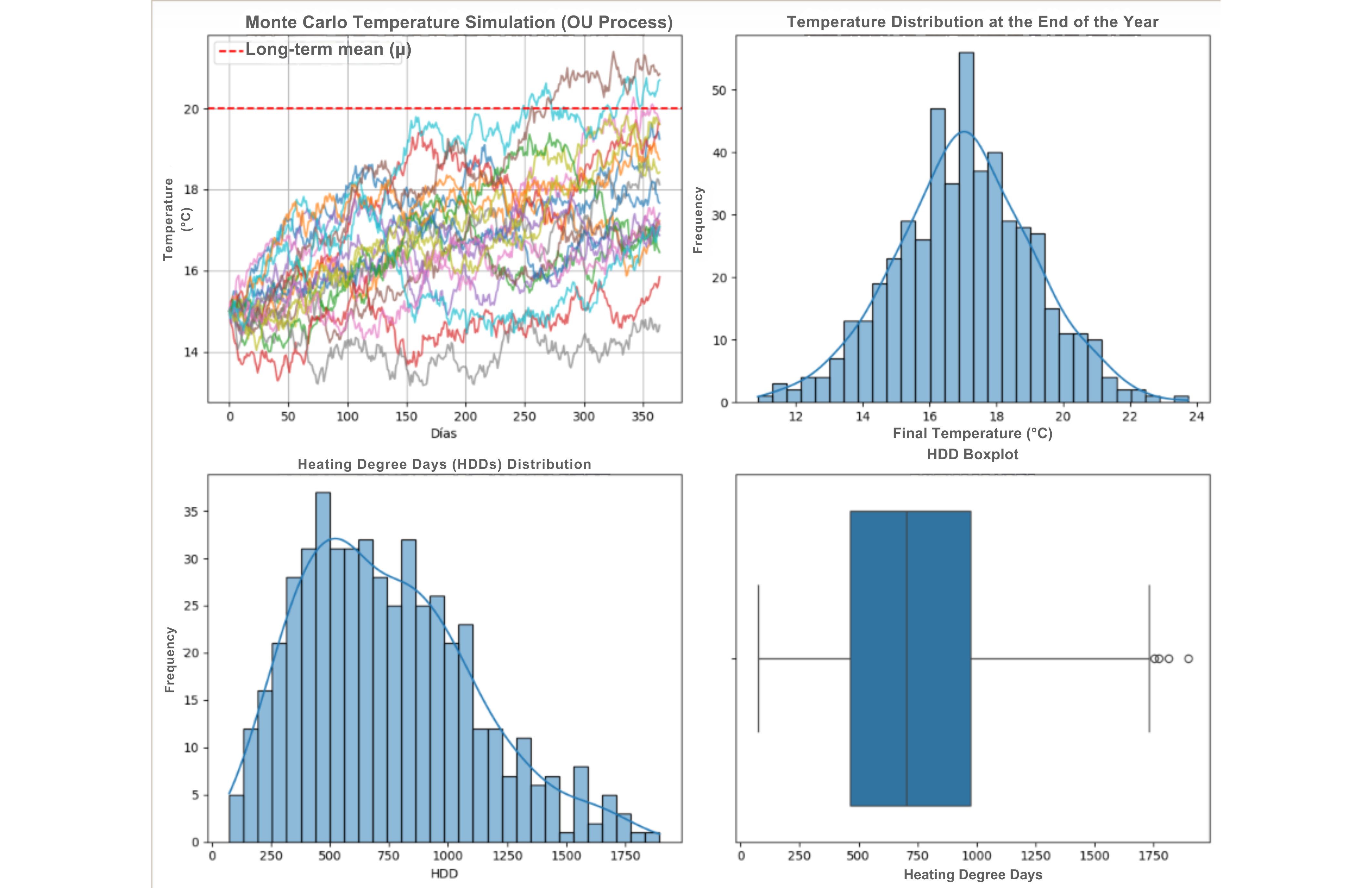
Figure 1: Monte Carlo simulation paths for temperature modeling

Weather Derivatives: Pricing Climate Uncertainty

Weather derivatives are OTC contracts tied to metrics like:

- Temperature (HDD/CDD indices)

- Precipitation (rainfall/swaps for agriculture)

- Wind speed (renewable energy hedging)

Key buyers: Utilities, insurers, agribusinesses hedging revenue volatility.

Modeling Temperature: Ornstein-Uhlenbeck Process

Temperature exhibits mean reversion—a core trait captured by the Ornstein-Uhlenbeck (OU) process:

dTₜ = θ(μ - Tₜ)dt + σdWₜ

Where:

- Tₜ = Temperature at time t

- μ = Long-term mean (e.g., 20°C for London)

- θ = Mean reversion speed (calibrated to historical data)

- σ = Volatility (higher in winter/summer)

import numpy as np
import matplotlib.pyplot as plt
import seaborn as sns

def simulate_temperature(T0, mu, theta, sigma, days, n_sims):
    """
    Simulates temperature paths using the Ornstein-Uhlenbeck (OU) process.
    """
    dt = 1 / 365  # Daily steps
    paths = np.zeros((n_sims, days))
    paths[:, 0] = T0

    for t in range(1, days):
        dW = np.random.normal(0, np.sqrt(dt), n_sims)
        paths[:, t] = paths[:, t - 1] + theta * (mu - paths[:, t - 1]) * dt + sigma * dW
    return paths

# Temperature parameters
T0, mu, theta, sigma = 15, 20, 0.5, 2.5
n_sims = 500  # More simulations
days = 365  # One year

# Generate simulations
np.random.seed(42)  # Reproducibility
temperature_paths = simulate_temperature(T0, mu, theta, sigma, days, n_sims)

# Calculate Heating Degree Days (HDDs)
HDDs = np.sum(np.maximum(18 - temperature_paths, 0), axis=1)

# Create figure with multiple plots
fig, axs = plt.subplots(2, 2, figsize=(12, 10))

# Plot 1: Temperature paths
for i in range(20):  # Only 20 paths for clarity
    axs[0, 0].plot(temperature_paths[i], alpha=0.7)
axs[0, 0].axhline(mu, color='red', linestyle='--', label='Long-term mean (μ)')
axs[0, 0].set_title('Monte Carlo Simulation of Temperature (OU Process)')
axs[0, 0].set_xlabel('Days')
axs[0, 0].set_ylabel('Temperature (°C)')
axs[0, 0].legend()
axs[0, 0].grid(True)

# Plot 2: Histogram of final temperatures
sns.histplot(temperature_paths[:, -1], bins=30, kde=True, ax=axs[0, 1])
axs[0, 1].set_title('Distribution of Final-Year Temperatures')
axs[0, 1].set_xlabel('Final Temperature (°C)')
axs[0, 1].set_ylabel('Frequency')

# Plot 3: Histogram of Heating Degree Days (HDDs)
sns.histplot(HDDs, bins=30, kde=True, ax=axs[1, 0])
axs[1, 0].set_title('Distribution of Heating Degree Days (HDDs)')
axs[1, 0].set_xlabel('HDD')
axs[1, 0].set_ylabel('Frequency')

# Plot 4: Boxplot of HDDs
sns.boxplot(x=HDDs, ax=axs[1, 1])
axs[1, 1].set_title('Boxplot of HDDs')
axs[1, 1].set_xlabel('Heating Degree Days')

# Adjust layout and show
plt.tight_layout()
plt.show()

Temperature exhibits mean reversion—a core trait captured by the Ornstein-Uhlenbeck

Convertible Bonds: Valuing Hybrid Securities

Convertible bonds combine debt features (coupon payments, principal repayment) with an embedded equity option allowing conversion into stock. Pricing is complex due to:

- Stock price evolution (modeled via geometric Brownian motion)

- Interest rate dynamics (e.g., Vasicek or CIR models)

- Optimal conversion strategy (American-style option feature)

import numpy as np
import matplotlib.pyplot as plt
import seaborn as sns

def simulate_gbm(S0, mu, sigma, T, dt, N):
    """
    Simulates stock price paths using Geometric Brownian Motion (GBM).
    """
    np.random.seed(42)
    paths = np.zeros((N, int(T / dt)))
    paths[:, 0] = S0

    for t in range(1, paths.shape[1]):
        dW = np.random.normal(0, np.sqrt(dt), N)
        paths[:, t] = paths[:, t - 1] * np.exp((mu - 0.5 * sigma**2) * dt + sigma * dW)
    return paths

def simulate_vasicek(r0, theta, mu, sigma, T, dt, N):
    """
    Simulates interest rate paths using the Vasicek model.
    """
    np.random.seed(42)
    paths = np.zeros((N, int(T / dt)))
    paths[:, 0] = r0

    for t in range(1, paths.shape[1]):
        dW = np.random.normal(0, np.sqrt(dt), N)
        paths[:, t] = paths[:, t - 1] + theta * (mu - paths[:, t - 1]) * dt + sigma * dW
    return paths

# Simulation parameters
S0, mu_stock, sigma_stock, T, dt, N = 100, 0.05, 0.2, 5, 1/252, 500
r0, theta, mu_rate, sigma_rate = 0.03, 0.1, 0.05, 0.02

# Generate simulations
stock_paths = simulate_gbm(S0, mu_stock, sigma_stock, T, dt, N)
rate_paths = simulate_vasicek(r0, theta, mu_rate, sigma_rate, T, dt, N)

# Create figure with multiple plots
fig, axs = plt.subplots(2, 2, figsize=(12, 10))

# Plot 1: Stock price simulation
for i in range(20):
    axs[0, 0].plot(stock_paths[i], alpha=0.7)
axs[0, 0].set_title('Monte Carlo Simulation of Stock Prices (GBM)')
axs[0, 0].set_xlabel('Days')
axs[0, 0].set_ylabel('Stock Price')
axs[0, 0].grid(True)

# Plot 2: Final stock price distribution
sns.histplot(stock_paths[:, -1], bins=30, kde=True, ax=axs[0, 1])
axs[0, 1].set_title('Distribution of Final Stock Prices')
axs[0, 1].set_xlabel('Final Stock Price')
axs[0, 1].set_ylabel('Frequency')

# Plot 3: Interest rate simulation
for i in range(20):
    axs[1, 0].plot(rate_paths[i], alpha=0.7)
axs[1, 0].set_title('Monte Carlo Simulation of Interest Rates (Vasicek)')
axs[1, 0].set_xlabel('Days')
axs[1, 0].set_ylabel('Interest Rate')
axs[1, 0].grid(True)

# Plot 4: Final interest rate distribution
sns.histplot(rate_paths[:, -1], bins=30, kde=True, ax=axs[1, 1])
axs[1, 1].set_title('Distribution of Final Interest Rates')
axs[1, 1].set_xlabel('Final Interest Rate')
axs[1, 1].set_ylabel('Frequency')

# Adjust layout and show
plt.tight_layout()
plt.show()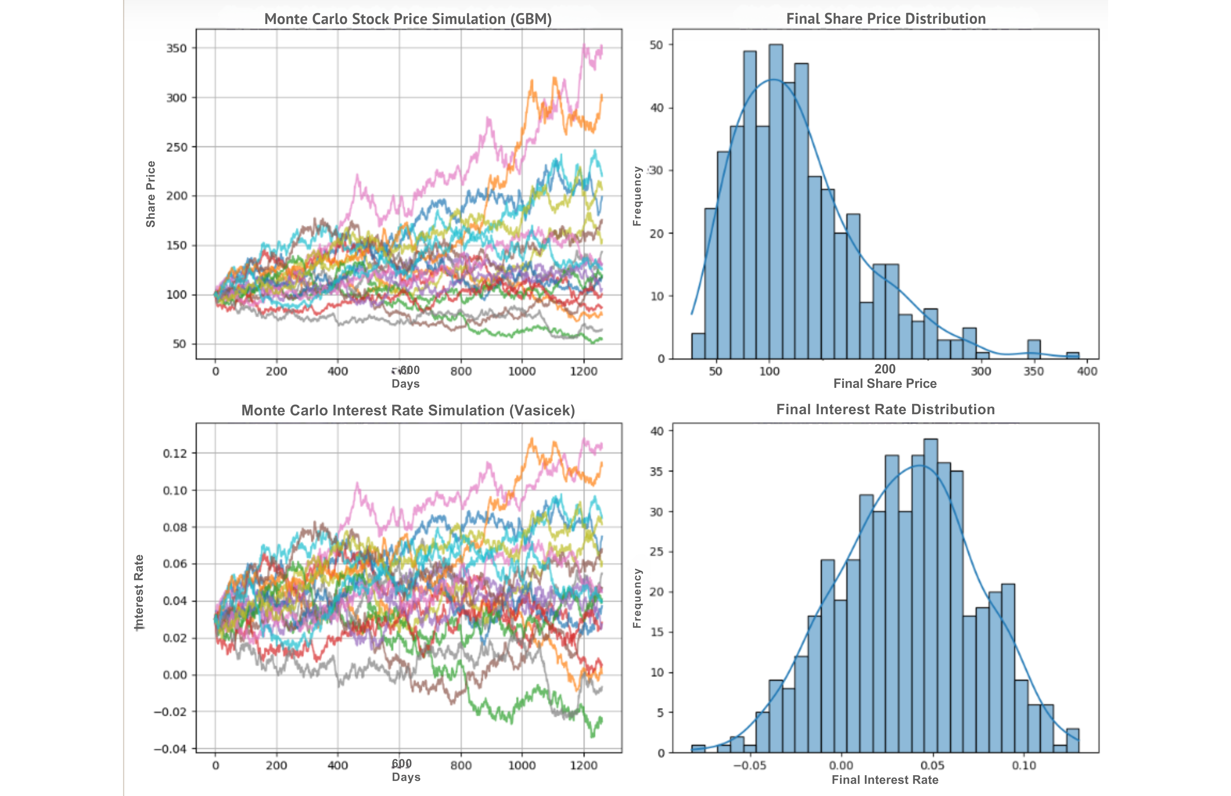

Convertible bonds combine debt features (coupon payments, principal repayment) with an embedded equity option allowing conversion into stock.

Key Takeaways

1. Monte Carlo simulations provide robust pricing for complex, path-dependent securities.

2. Weather derivatives benefit from stochastic temperature modeling (OU process).

3. Convertible bonds require joint simulation of stock prices and interest rates.

4. Python implementation allows flexible scenario analysis and risk assessment.

Monte Carlo methods are indispensable for modern financial engineering, enabling precise valuation of structured products in uncertain environments. By integrating market data and advanced calibration techniques, analysts can derive actionable insights for investment and risk management.