PCA in Action: From Commodities to Trading

Introduction: The Power of Principal Component Analysis

Principal Component Analysis (PCA) is a statistical technique used to reduce data dimensionality while preserving key information. In financial markets, PCA is instrumental in extracting dominant risk factors from complex datasets, making it invaluable for:

✔ Commodity derivatives pricing: Identifying key market drivers

✔ Dispersion trading: Decomposing index volatility into constituent stock volatilities

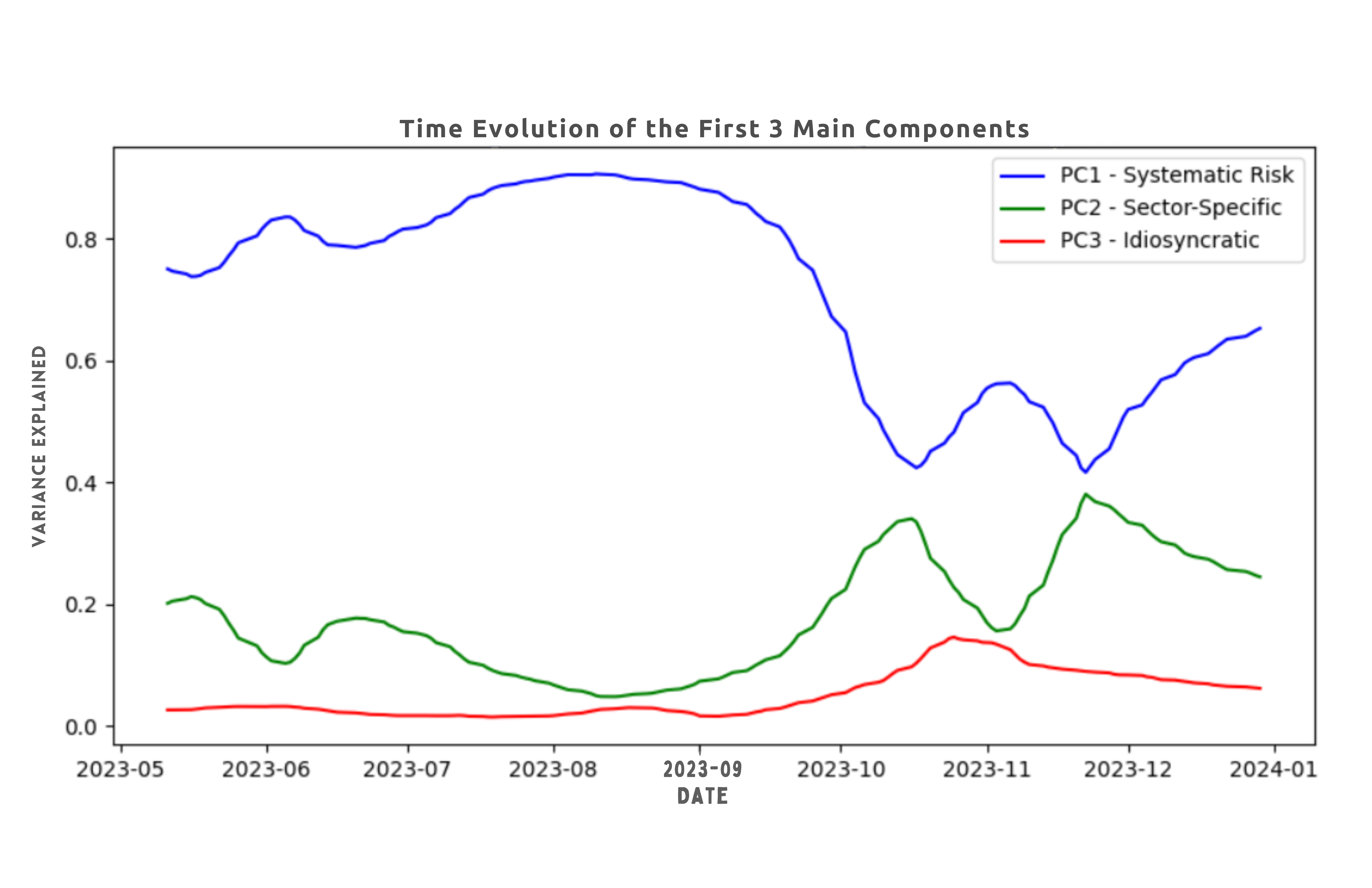
Figure 1: PCA variance explained in commodity markets

PCA in Commodity Derivatives Pricing

Commodity derivatives are widely used for risk management. PCA helps identify principal factors influencing prices:

- Macroeconomic indicators (inflation, GDP growth, rates)

- Supply/demand shocks (weather, geopolitics)

- Energy prices (oil/gas correlations)

import numpy as np
import matplotlib.pyplot as plt
import seaborn as sns
import yfinance as yf
from sklearn.decomposition import PCA

# Download historical price data for commodities from Yahoo Finance
tickers = ["GC=F", "CL=F", "SI=F", "HG=F", "ZC=F"]  # Gold, crude oil, silver, copper, and corn
data = yf.download(tickers, start="2023-01-01", end="2024-01-01")

# Check if 'Close' prices are present in the data
data = data.get('Close')
if data is None:
    raise ValueError("No 'Close' data found in the Yahoo Finance download.")

# Remove rows with NaN values
data.dropna(inplace=True)

# Apply PCA
pca = PCA()
pca.fit(data)
explained_variance = pca.explained_variance_ratio_

# Plot the explained variance with better clarity
plt.figure(figsize=(8, 5))
sns.barplot(x=np.arange(1, len(explained_variance) + 1), y=explained_variance * 100, palette='viridis')
plt.xlabel('Principal Component (PCA)')
plt.ylabel('Explained Variance (%)')
plt.title('Explained Variance by Each Principal Component')
plt.xticks(np.arange(len(explained_variance)), labels=[f'PC{i+1}' for i in range(len(explained_variance))])
plt.show()

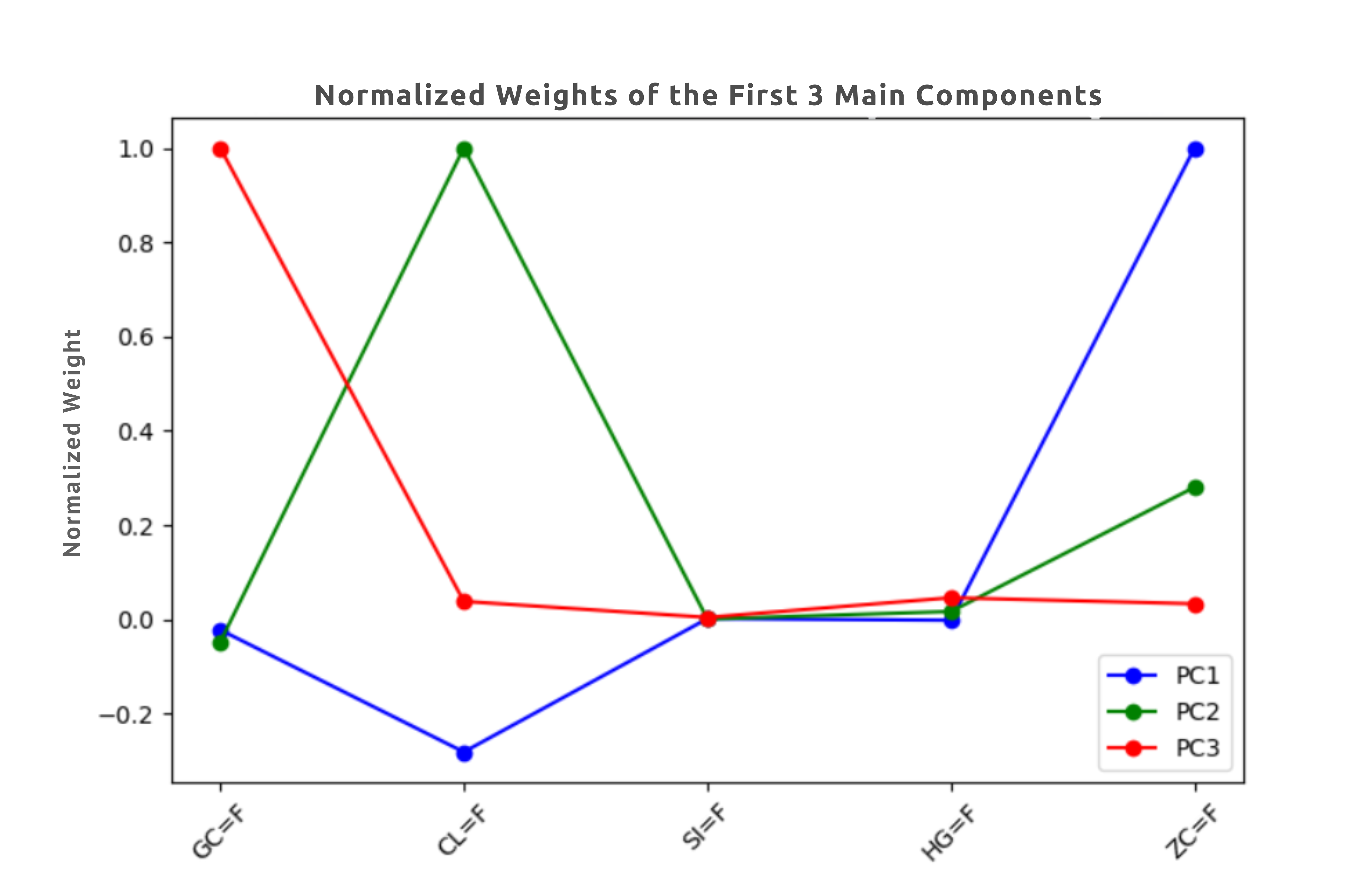
# Plot the coefficients of the first 3 principal components, scaled for better interpretation
plt.figure(figsize=(8, 5))
indices = np.arange(len(tickers))
colors = ['b', 'g', 'r']

for i in range(3):
    plt.plot(
        indices,
        pca.components_[i] / np.max(np.abs(pca.components_[i])),
        marker='o',
        linestyle='-',
        label=f'PC{i+1}',
        color=colors[i]
    )

plt.xticks(indices, tickers, rotation=45)
plt.xlabel('Commodities')
plt.ylabel('Normalized Weight')
plt.title('Normalized Weights of the First 3 Principal Components')
plt.legend()
plt.show()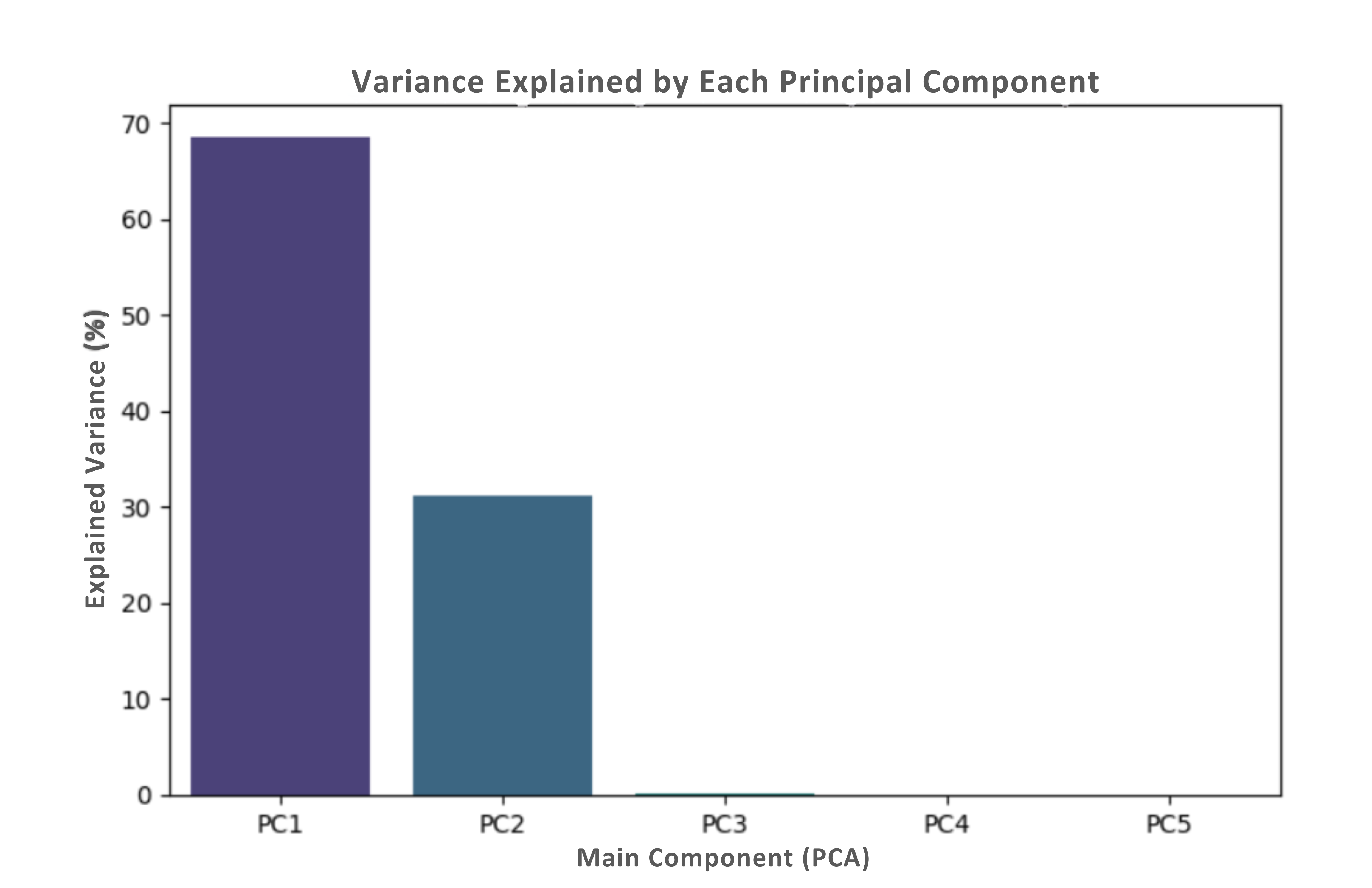

Macroeconomic indicators (inflation, GDP growth, rates)

Supply/demand shocks (weather, geopolitics)

Key PCA Insights

1. PC1 (captures the highest variance): Broad macroeconomic influences

2. PC2: Sector-specific factors

3. PC3: Idiosyncratic shocks

4. PC4+ (minor variance): Additional noise or less significant patterns

The analysis considered multiple principal components, with the first three explaining most of the variance. However, up to five components were visualized for a better understanding of the data structure.

PCA for Dispersion Trading

Dispersion trading exploits differences between index and single-stock volatilities. PCA helps:

✔ Quantify systematic vs. idiosyncratic risk

✔ Identify mispriced volatility components

✔ Optimize hedging ratios

import numpy as np
import matplotlib.pyplot as plt
import seaborn as sns
import yfinance as yf
from sklearn.decomposition import PCA

# Download historical stock price data for selected S&P 500 companies from Yahoo Finance
tickers = ["AAPL", "MSFT", "GOOGL", "AMZN", "META", "TSLA", "NVDA", "BRK-B", "JPM", "V"]
data = yf.download(tickers, start="2023-01-01", end="2024-01-01")

# Check if 'Close' prices are present in the data
data = data.get('Close')
if data is None:
    raise ValueError("No 'Close' data found in the Yahoo Finance download.")

# Remove rows with missing values
data.dropna(inplace=True)

# Apply rolling PCA with a 90-day window
window_size = 90
pca_results = []
dates = []

for i in range(len(data) - window_size + 1):
    window_data = data.iloc[i:i + window_size]
    pca = PCA()
    pca.fit(window_data)
    pca_results.append(pca.explained_variance_ratio_[:3])
    dates.append(data.index[i + window_size - 1])

# Convert PCA results to a NumPy array for plotting
pca_results = np.array(pca_results)

# Plot the evolution of the first 3 principal components over time
plt.figure(figsize=(10, 5))
plt.plot(dates, pca_results[:, 0], label='PC1 - Systematic Risk', color='b')
plt.plot(dates, pca_results[:, 1], label='PC2 - Sector-Specific', color='g')
plt.plot(dates, pca_results[:, 2], label='PC3 - Idiosyncratic', color='r')
plt.xlabel('Date')
plt.ylabel('Explained Variance')
plt.title('Temporal Evolution of the First 3 Principal Components')
plt.legend()
plt.show()

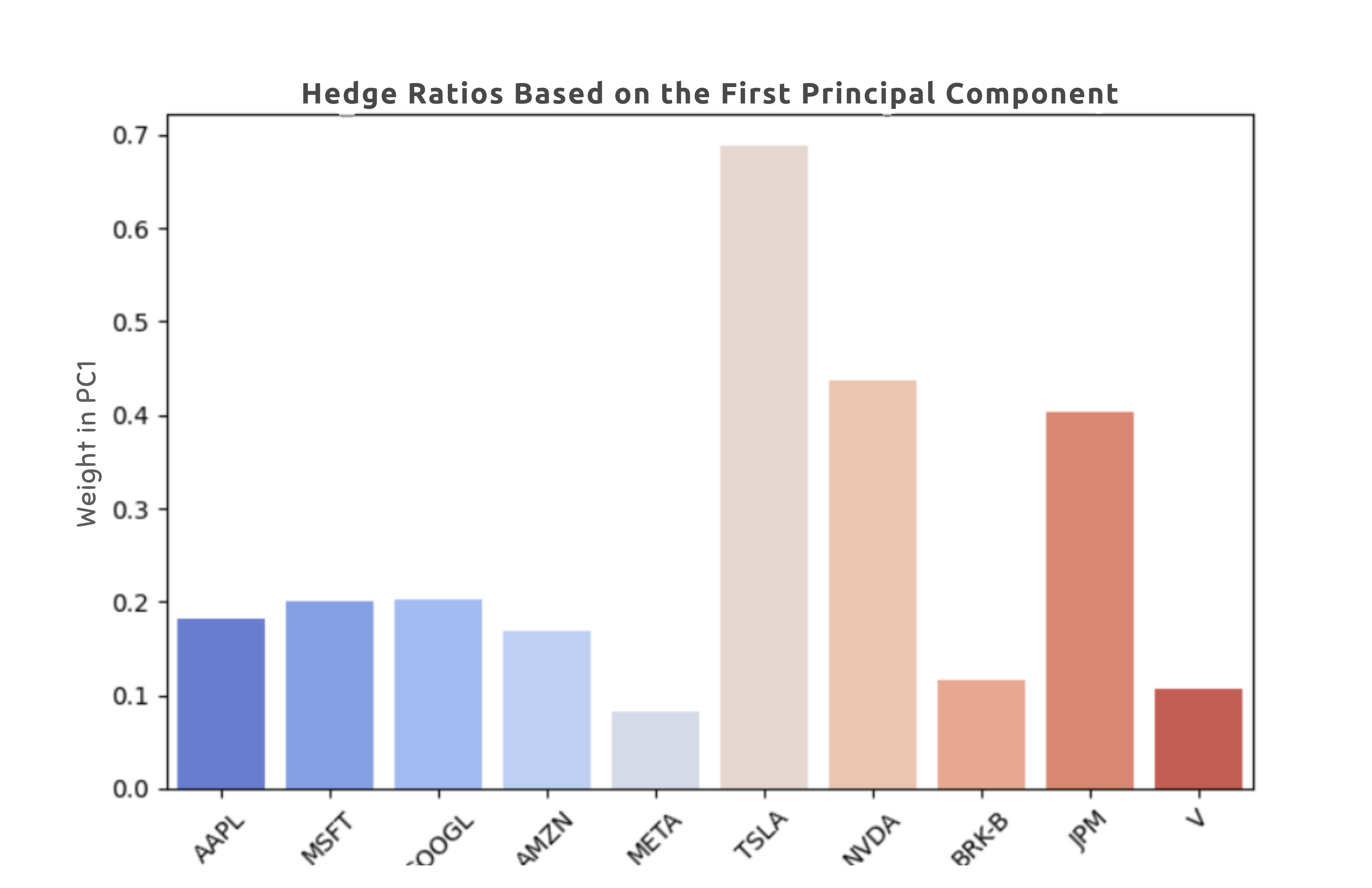
# Fit PCA on the entire dataset to extract hedge ratios from the first principal component (PC1)
pca = PCA()
pca.fit(data)
hedge_ratios = pca.components_[0]

# Plot hedge ratios
plt.figure(figsize=(8, 5))
sns.barplot(x=tickers, y=hedge_ratios, palette='coolwarm')
plt.xlabel('Stocks')
plt.ylabel('Weight in PC1')
plt.title('Hedge Ratios Based on the First Principal Component')
plt.xticks(rotation=45)
plt.show()

Rolling PCA windows for dynamic factor exposure

PC1 as hedge ratio for index products 3. Idiosyncratic components for pair trading opportunities

Practical Applications

1. Rolling PCA windows (60-90 days) for dynamic factor exposure

2. PC1 as hedge ratio for index products

3. Idiosyncratic components for pair trading opportunities

Conclusion

PCA provides a robust framework for identifying market drivers in both commodity pricing and dispersion trading. By decomposing volatility into systematic and idiosyncratic components, traders can develop more effective risk models and capture alpha opportunities.